LAPSUS-LS model Landsliding

For modelling soil redistribution in a catchment where shallow landsliding is the dominant process determining landscape evolution, LAPSUS-LS, a landslide component, was developed by Claessens et al. (2005, 2007) and added to the original LAPSUS structure. This component calculates (1) landslide risk for each individual grid cell, and (2) trajectories of failed slope material that travels downslope as debris flows (Claessens et al., 2005, 2007).

Case Studies: » New Zealand, Taiwan, Uganda

Technical Information

Montgomery and Dietrich (1994), based on earlier formulations proposed by O'Loughlin (1986), combined a contour based steady state hydrologic model with a deterministic infinite slope stability model to delineate areas prone to landsliding due to surface topographic effects on hydrologic response. Our approach is based on this method but has two differences (as in Pack et al., 2001):

1) The cohesion term is retained in the infinite slope stability model to account for differences in soil cohesion between geological formations and additional strength by root reinforcement for different vegetation types.

2) We use grid-based rather than contour based DEM methodology.

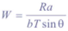
Next to topography, subsurface flow and combined cohesion are recognized as most important factors controlling shallow landsliding. Relative wetness W is the ratio of local steady state rainfall flux to the flux at soil profile saturation. Based on work of O’Loughin (1986) and Moore et al. (1988), a steady state hydrologic response model defines W as:

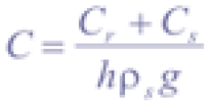
where R (md-1) is steady state rainfall recharge, a (m2) is the contributing drainage area, b (m) the unit contour length (i.e. gridsize), T (m2d-1) saturated soil transmissivity, and θ (°) local slope angle. The range of values for wetness W is between 0 and 1, since any excess of 1 is assumed to form overland flow. Combined cohesion C can be interpreted as the relative contribution to slope stability of the cohesive forces (Claessens, 2005), and is defined as follows: 

where Cr (Nm-2) and Cs (Nm-2) are root cohesion and soil cohesion respectively, h (m) is perpendicular soil thickness, ρs (gcm-3) is wet soil bulk density, and g is the gravitational acceleration constant (9.81ms-2). For calculation of the factor of safety FS, which is the ratio of total shear strength to total shear stress, (1) and (2) are combined:

with ρw (gcm-3) the density of water, and Ø (°) effective angle of internal friction of the soil. The minimum steady state rainfall necessary to cause slope failure, named critical rainfall Qcr (md-1), can be determined by substituting equation (1) in (3), equating FS to 1 and solving for R.

Qcr can be interpreted as a prediction of relative potential for landslide initiation (Borga et al., 1998). Some elements are unconditionally stable (e.g. flat areas) or unstable (e.g. bedrock outcrops). When,

an element is predicted to be unconditionally stable, even when saturated. Unconditionally unstable elements have,

When failed, material starts moving downslope as a debris flow. LAPSUS_LS calculates the trajectories of failed slope material as follows: unstable soil material is accumulated by the debris flow during the erosional phase. Based on works by Johnson and Rodine (1984, as in Claessens, 2005) and e.g. Burton and Bathurst (1998) the amount of eroded material S (m) is calculated as:

where ρs (kNm-3) is bulk density,  α (°) is the minimum local slope for debris flow movement, and a (m2) corrects for dimensions. Thus soil geotechnical properties and local slope define S. Erosion stops where the gradient falls below a certain slope angle α (depending on local typical landslide dimensions) and the transported material will be deposited over a cell-distance D (-):

where b (m) is gridsize and R (m) is the runout distance:

where the elevation difference Δy (m) between the head of the slide and the point where deposition begins (as an indicator for debris flow momentum) and an empirically derived fraction φ set at 0.4 (Burton and Bathurst, 1998) define the distance over which material will be deposited. Deposition follows a ‘double’ multiple flow methodology, based on the multiple flow concept by Quinn et al. (1991, as in Claessens 2005).